PREVIOUSGnuPlot,Python绘图模板整理
NEXTWannierTools 编译
QuanSheng Wu
École Polytechnique Fédérale de Lausanne (EPFL), Switzerland
Constructed on October 30, 2019
High-quality Wannier functions (WFs) are very useful for physical properties calculations after we obtained the self-consistent charge density from the first-principle calculations. However, for the beginners, it’s not easy to obtain good WFs. Here we would like to introduce a standard way to construct high-quality Wannier functions with first-principle software package and software Wannier90. Here we don’t focus on constructing maximum localized Wannier functions (MLWFs). We only want to construct a good tight-binding model based on WFs that are able to reproduce the band structure in the energy range we are interested in. Here are four criterions of high-quality WFs.
There are three important steps to reach four criterions.
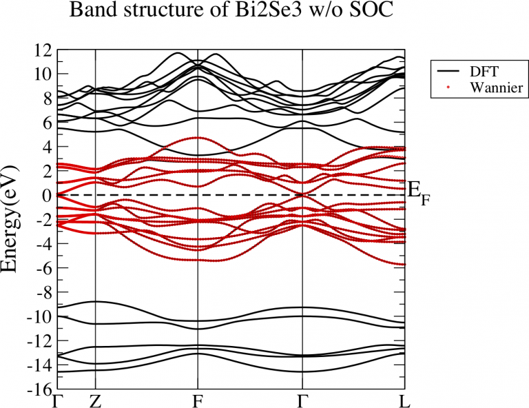
I would like to take Bi2Se3 as an example. In order to save the computation cost, we don’t take into account the spin-orbit coupling (SOC) effect.
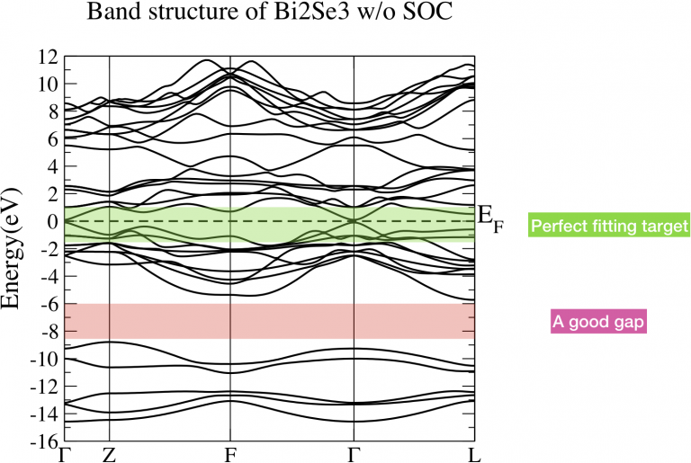
Let’s perform energy band analysis first. Fig 1 is the band structure of Bi2Se3 without considering SOC. The green shaded part is the energy range which we care about. We want to construct a tight binding model which can well reproduce the energy bands in that interested range. However, those band is connected with other bands below and above. Noticeably, there is a big gap around -8.4eV and -6eV. This is a good sign since the bands below this gap is not hybridized with the bands we are interested in. In this case, those bands below the gap are not necessary to be presented in our tight binding model. Eventually, the number of WFs reduce. It fulfills the fourth criterion.
After a first glance of the band structure, we still have to figure out what is the character of the bands in the interested energy range and figure out which bands are highly hybridized with them. This step is called “fatband analysis” where we need to project the atomic orbital onto the Bloch wave functions which is called the projected weight. We project the Bloch wave functions onto the s, p, d atomic orbitals of Bi and Se. The results are shown in Fig 2. Fig 2(a) and (d) show that the energy bands between [-15, -8]eV are dominated by the s orbital of Bismuth and Selenium. Fig 2 (c) and (f) show that the d orbitals of Bi and Se are located above 5eV. Fig 2 (b) and (e) show that the energy range [-6, 5] eV is dominated by p orbitals of Bi and Se. And our interested energy range, indicated as green shade in Fig 1, is in this energy range. Although there is band overlap between p and d orbitals at around 4eV, we still can omit the contribution from d orbitals since they are not high hybridized with p orbitals and can be shifted away through some deformation of the band structure.
After the “fatband analysis”, we choose p orbitals of Bi and Se as projectors for WFs. Then there will be (2 Bi atoms)*(3 p orbitals)+(3 Se atoms) *(3 p orbitals)=15 atomic orbitals, totally 15 WFs without SOC.
begin projections
Bi : p
Se : p
end projections
The disentanglement window is a window to extract the target bands. There are two rules to set this window. 1) Not only the target bands should be included in this window, but also the major weight of the projectors should fall into this window. 2) This window should as small as possible in order to reduce the computational cost. Fig 3 gives three choices of the window marked as colored shade. Fig 3(a) is the right choice. Fig 3(b) is a very bad choice since there is one missing band, marked by dashed circle, whose weight comes from the projectors (See Fig 4b and 4e). If this weight is missing, then the spread of the WFs could become large. Fig 3(c) shows a not good choice since it contains unnecessary bands which don’t contain projector’s character.
The frozen window is a window used for disentanglement procedure. The Bloch states will not rotate with other bands out of this window. There are three rules for choosing froz_win. 1) In froz_win, there should be no weights (contributions) coming from other orbitals besides the projectors. 2) The energy range purely coming from the projectors should be included in the froz_win. 3) froz_win should be as large as possible. Fig 4 shows three choices. (a) is a good choice since it fulfill three rules . (b) is a wrong choice since it breaks the first rule. (c) is correct choice but not a perfect one since it doesn’t follow rule 2 and 3.
After the above procedure, you shall get very good WFs with high possibility. Fig 5 shows the band structure comparison between DFT (black lines) and Wannier interpolation (red dots). It shows perfect agreement.
In the end, we would like to share some other tips.